October 28, 2014
Skewing around, Part 1
A while ago, a friend of mine asked for help analyzing a continuous integer stream of values spread across a large range. He wanted a way to determine if a subset of values appeared more frequently than the rest. He didn’t necessary want to know what those values were, just the degree to which the value occurrence frequencies were similar. Now, my friend didn’t have just one stream to analyze, there were hundreds, perhaps thousands. So, the solution had to use minimal compute and memory resources. He also wanted the skew estimated in real-time as the streams were received.
Lucky for him, I had just completed Stanford’s Mining Massive Datasets class (CS246) that covered, among other things, using probabilistic online algorithms to estimate a data stream’s frequency moments.
Determining a population’s diversity is a well studied problem that has applications in many fields including ecology, and demography. Many quantitative measures exist for representing diversity including one called the second frequency moment which is related to sample variance. For a sequence of integers \(A = (a_1, a_2, \ldots, a_m) \) where \( a_i \in (1,2,\ldots,n) \) and \( m_i \) is the number of times the value \( i \) appears in the stream, the second freqency moment is defined as,
To see how this works, consider a stream of 20 integers with 4 unique values. When each value appears an equal number of times, \(F_2\) is,
In the maximum skew case with appearance counts of 15, 2, 1, and 1, \(F_2\) will be,
As this simple example illustrates, the second frequency moment is minimized when the distribution is even and maximized when the distribution is the most skewed. In essence, it reflects how “surprising” a stream’s values are. For this reason, the second frequency moment is sometimes called the “surprise number”.
The surprise number is easy to calculate but requires keeping a count for each distinct value in the stream. This can lead to excessive memory consumption for streams with many, many unique values - exactly like my friend’s situation.
In a 1996 paper, Alon, Matias, and Szegedy (AMS) presented a space efficient, on-line algorithm for estimating frequency moments. The algorithm is deceptively simple. For now, assume that the integer sequence \(A\) from earlier has a known length. A subset of \(P\) stream positions are chosen a-priori with uniform probability. At each of the selected positions in stream, the integer value is recorded along with a counter initialized to 1. From that point onward, the counter is incremented each time the recorded value appears in the stream. At the end of the stream, there are \(P\) counters that can be used to estimate the surprise number by calculating,
For example, consider the integer stream ( 6, 6, 1, 5, 4, 4, 10, 3, 3, 2, 10, 10, 9, 2, 10) and selected positions 1, 5, 13, and 14. At the end of the stream, the four AMS counters are
| Position | Value | Count |
|---|---|---|
| 1 | 6 | 2 |
| 5 | 4 | 2 |
| 13 | 9 | 1 |
| 14 | 2 | 1 |
The actual second frequency moment is,
and the AMS algorithm’s estimate is,
For this simple example the AMS estimate has a relative error of 16% but, in general, the algorithm achieves better accuracy with more counters. To illustrate this, the following chart plots the AMS algorithm’s accuracy for simulated streams of 100000 integers with 1000 unique values (the R code for the simulation is included at the end of this post),
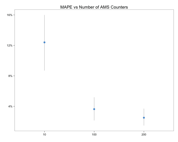
The dots and vertical lines respectively represent the mean average percent error (MAPE) and 95% confidence interval across ten trials for each case. This simple simulation shows how the relative error decreases as the number of AMS counters increases and generally converges to within 5%. It also shows the algorithm’s sensitivity to the number of unique values in the stream.
The observant reader may notice that it’s possible for multiple AMS counters to track the same value. This is OK, each counter is basically an independent estimate of the second frequency moment so these redundant counters can simply be averaged together.
This is pretty cool. But what about infinite streams? AMS relies on the uniform selection of stream positions to sample. How can that be done if the stream is continuous? The intuitive solution is to periodically replace an existing counter with a new one later in the stream. The trick, is deciding when to do the replacements to maintain the uniform selection probability.
This turns out to be pretty simple. To start, create AMS counters for the first \(P\) elements. For each subsequent stream element, replace an existing counter with probability \(P/(i+1)\), where \(i\) is the stream’s present length. The actual counter replaced is chosen with equal probability. Mathematically, this all works out such that the counter sample positions have equal probability at each point in the stream.
The AMS algorithm can be used to estimated higher order moments as well. For a thorough discussion of the algorithm and associated mathematical proofs, see Section 4.5 of the book Mining of Massive Datasets.
Getting back to my friend’s problem, the AMS algorithm provided a way to estimate a stream’s skew. However, comparing the skew of different streams is difficult as the second frequency moment’s absolute value can vary greatly based on the stream length, etc. Therefore, I needed a more reliable means for comparing streams which will be the subject of the next post.
Here is the AMS simulation R code.
    library(Hmisc)
    library(ggplot2)
    library(scales)
    library(ggthemes)

    set.seed(1234567)

    stream.max     <- 100000
    num.unique     <- c(1000)
    stream.lengths <- c(100000)
    ams.counters   <- c(10, 100, 200)

    test.cases <- expand.grid(l=stream.lengths,
                              c=ams.counters,
                              n=num.unique)

    test.cases <- test.cases[rep(1:nrow(test.cases), 10),]


    ams.test <- function(l,c,n) {

     values <- sample.int(stream.max, n)
     stream <- sample(values, l, replace=TRUE)
     indxs  <- sort(sample(1:l, c))

     counts <- sapply(indxs, function(i) {
                         sum(stream[i:length(stream)] == stream[i])
                      })

     actual    <- sum(table(stream)^2)
     estimated <- l/c * sum(2*counts -1)

     data.frame(l=l,c=c, n=n, actual=actual, AMS=estimated)
    }

    results <- Reduce(rbind,
                      apply(test.cases,1,
                      function(t) { ams.test(t["l"],t["c"], t["n"])}))

    results$l <- as.factor(format(results$l, scientific=FALSE))
    results$c <- as.factor(results$c)
    results$n <- factor(results$n, levels=num.unique,
                        labels=paste(num.unique, "Unique Values"))

    results$rerror <- abs(results$actual - results$AMS) /
                      results$actual

    ggplot(results, aes(c, rerror,group=n)) +
       stat_summary(fun.data="mean_cl_boot", color="gray") +
       stat_summary(fun.y=mean, geom="point", size=3,
                    color=ggthemes_data$few$medium["blue"]) +
       labs(title="MAPE vs Number of AMS Counters", x="",y="") +
       scale_y_continuous(labels = percent) +
       theme_few()
Tags: MachineLearning , Streams , R