Although I’m late to the start, I’ve been working on the Kaggle Toxic Comment Challenge. The dataset only contains about 560K comments. Before trying a deep learning model, I was curious to see how well a relatively simple approach might do. At the same time, I still wanted to use word embeddings to maximize generalization to unseen text.

The Coursera Deep Learning Sequence Models class described summarizing documents by averaging over each word’s embedding vector. Some quick research led me to this paper that, in part, describes using the TF-IDF weighted sum of embedding vectors instead. That seemed cool so I decided to give it a try.

I’ll describe how I did this using a subset of the 20 newsgroups dataset. The scikit-learn package provides a helper function to do this (note that you may want to change the data_home parameter).

from sklearn.datasets import fetch_20newsgroups
news_train = fetch_20newsgroups(subset='train', categories=['sci.space','rec.autos'], data_home='~/local/tmp')

This data set has 1187 documents, 594 from rec.autos and 593 from sci.space. Next, we’ll load the spaCy Python package and its medium-size English language model which includes pre-computed Glove embedding vectors. See the spaCy page for instructions on downloading the language model.

import spacy

nlp  = spacy.load('en_core_web_md')

With spaCy loaded, the newsgroup documents can be lemmatised.

def keep_token(t):
    return (t.is_alpha and 
            not (t.is_space or t.is_punct or 
                 t.is_stop or t.like_num))

def lemmatize_doc(doc):
    return [ t.lemma_ for t in doc if keep_token(t)]

docs = [lemmatize_doc(nlp(doc)) for doc in news_train.data]

Next, the Gensim package can be used to create a dictionary and filter out stop and infrequent words (lemmas).

from gensim.corpora import Dictionary
from gensim.models.tfidfmodel import TfidfModel
from gensim.matutils import sparse2full

docs_dict = Dictionary(docs)
docs_dict.filter_extremes(no_below=20, no_above=0.2)
docs_dict.compactify()

This process yields a vocabulary with 1191 words. Gensim can again be used to create a bag-of-words representation of each document, build the TF-IDF model, and compute the TF-IDF vector for each document.

import numpy as np

docs_corpus = [docs_dict.doc2bow(doc) for doc in docs]
model_tfidf = TfidfModel(docs_corpus, id2word=docs_dict)
docs_tfidf  = model_tfidf[docs_corpus]
docs_vecs   = np.vstack([sparse2full(c, len(docs_dict)) for c in docs_tfidf])

The result, docs_vecs, is a matrix with 1187 rows (docs) and 1191 columns (TF-IDF terms). Next, we use spaCy to get the 300 dimensional Glove embedding vector for each TF-IDF term.

tfidf_emb_vecs = np.vstack([nlp(docs_dict[i]).vector for i in range(len(docs_dict))])

The tfidf_emb_vecs matrix has 1192 rows (terms) and 300 columns (Glove vectors). To get a TF-IDF weighted Glove vector summary of each document, we just need to matrix multiply docs_vecs with tfidf_emb_vecs.

docs_emb = np.dot(docs_vecs, tfidf_emb_vecs) 

As expected, docs_emb is a matrix with 1187 rows (docs) and 300 columns (Glove vectors).

To get sense of how well these document summaries do, we can use PCA to reduce the dimensionality,

from sklearn.decomposition import PCA
docs_pca = PCA(n_components=8).fit_transform(docs_emb)

and then use t-sne to project the vectors to 2D.

from sklearn import manifold

tsne = manifold.TSNE()
viz = tsne.fit_transform(docs_pca)

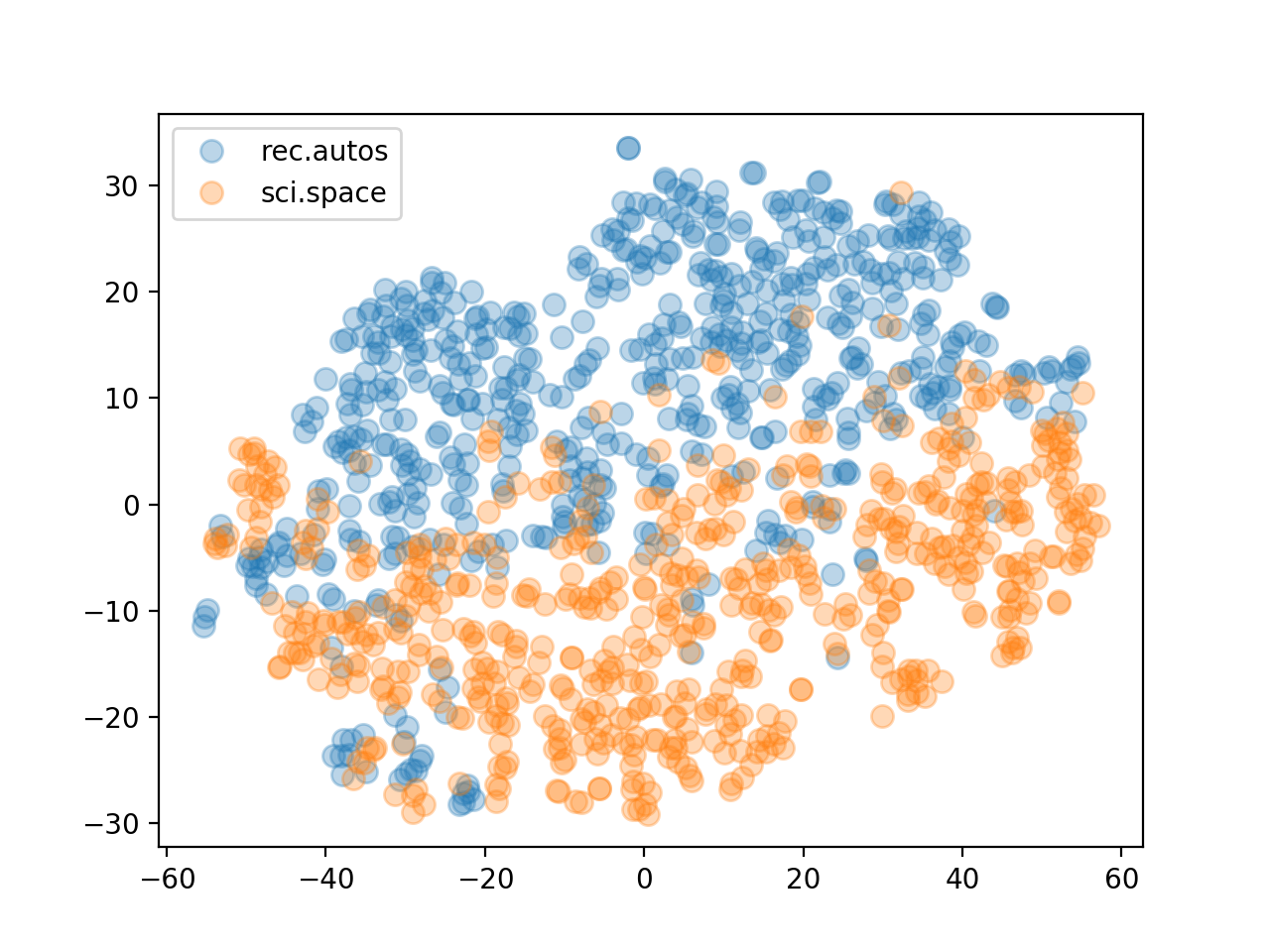
Plotting with matplotlib…

import matplotlib.pyplot as plt

fig, ax = plt.subplots()
ax.margins(0.05) 

zero_indices = np.where(news_train.target == 0)[0]
one_indices = np.where(news_train.target == 1)[0]

ax.plot(viz[zero_indices,0], viz[zero_indices,1], marker='o', linestyle='', 
        ms=8, alpha=0.3, label=news_train.target_names[0])
ax.plot(viz[one_indices,0], viz[one_indices,1], marker='o', linestyle='', 
        ms=8, alpha=0.3, label=news_train.target_names[1])
ax.legend()

plt.show()

Produces the following plot which shows that the TF-IDF weighted Glove vectors did a decent job of separating the documents.

I did some additional feature engineering to further improve separability for the Kaggle competition. After fitting an SVM binary classification model for each label, I was able to achieve a score of 0.9470 on the mean column-wise ROC AUC metric used by the competition. While not bad, it’s far from the best leaderboard scores. I may experiment some more with weighted embedding vectors but I fear too much information is lost in the summarizing to get to the top of the board.